Sheet Name Code

What is Sheet Name Code Excel Formula?

The Sheet Name Code in Excel is a formula that effectively displays the sheet's name in a cell as it retrieves the name of the current worksheet. This can be particularly useful for different purposes, such as creating templates, automating reports, and optimizing data analysis. 

Worksheets are collections of cells arranged and stacked together on top of one another, resembling rows and columns. Worksheets play an integral role in the Workbooks by separating one type of data from another. 

For example, assume you are preparing a Discounted Cash Flow Model for Apple Inc. You can input assumptions in one spreadsheet, prepare the three-statement model in another, and create a DCF model and summary in the other two sheets.

What do you think is the advantage of representing data in different spreadsheets?

Firstly, it helps to organize data appropriately. Thus, it is easier to find the information whenever you revisit the data source than when everything is crammed into one sheet.

Think of ants for a second. They build complicated tunnels, yet they can find the path to various chambers and food storage rooms due to their organized efforts.

Secondly, each spreadsheet can be customized as per the user's requirement. For example, changing the fill color, removing gridlines, freezing panes, changing the font size and color, etc.

Lastly, because it is free! Well, technically, you did pay a fee to Microsoft for the Excel software, so why not fully leverage God's power?

Now you know why to represent data in different spreadsheets, we will show how you can return the spreadsheet name in a selected cell. 

Later we will explain why you need spreadsheet names.

Sheet Name Code: Extract the Sheet Name using the formula

Suppose you are working on a dataset consisting of hundreds of different spreadsheets. You must type in the sheet name in each of those spreadsheets at the top since you need to print those in PDF format.

The easiest method is to copy the sheet name and paste it into the desired cell. But wait! There are still 99 more spreadsheets to go. It would take much longer to go through all the spreadsheets and copy the names in selected cells.

Here, we can use the MID, FIND, and CELL function combination that captures the spreadsheet name in the selected cell.

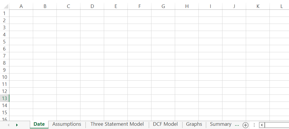
Suppose you have different spreadsheet names, as illustrated below:

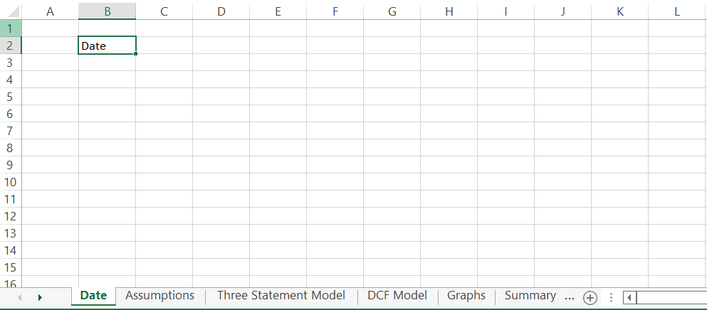
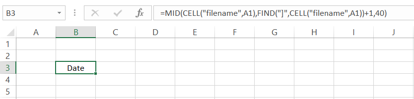
Let's say we want the sheet name in cell B2. We will use the formula =MID(CELL("filename",A1),FIND("]",CELL("filename",A1))+1,40) in cell B2, which gives the result:

However, you cannot copy the formula in each sheet so that it represents the sheet name in cell B2 of each spreadsheet.

Instead, all you need to do is copy cell B2 > Right-click on any worksheet > Select all Sheets, which selects all the cells as illustrated below:

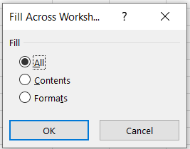
Next, click Home > Fill in Editing Section > Across Worksheets > Fill type as 'All.'

If you check any spreadsheet, you will find that all the B2 cells have respective sheet names.

How does the Sheet Name Code Excel formula work?

To understand how the formula works, let's break it down into simple components:

• The most important thing you need to remember is to save the file before working further. If you input the formula directly, you will get a #VALUE! Error.
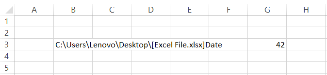
• The piece used twice in the formula is =CELL("filename",A1), which returns the complete path where the file is saved.

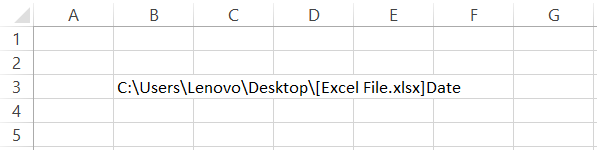
• We get the result as C:\Users\Lenovo\Desktop\[Excel File.xlsx]Date in the selected cell. Next, the FIND function identifies the ‘]’ and returns its position based on the text string equal to 41.
• We add 1 to FIND("]",CELL("filename",A1))+1 since we want the starting position of the substring to begin with the sheet name, which in this case is ‘Date.’

• Finally, we combine both the results in the MID function, such that the complete formula is =MID(CELL("filename",A1),FIND("]",CELL("filename",A1))+1,40). 
• The num_chars argument equals 40 since the minimum number of characters you can use to rename a worksheet is 31. Of course, you can input a number greater than this, and the function will still work properly.

Extract Sheet Name in a single worksheet

There won't always be a scenario where you want the names in the spreadsheet.

What if you want all the sheet names in one spreadsheet itself?

In this case, we can use the 'Define Name' function and a formula to generate a list of all the spreadsheets in the workbook.

First, click on Formulas > Define Name, which will open up a window as illustrated below:

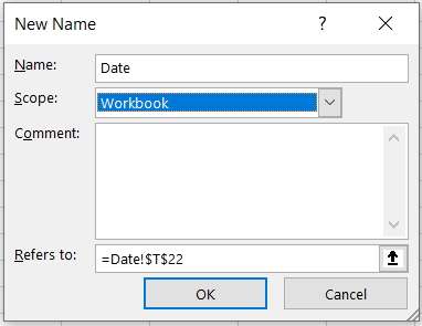
Here, we assign a name to the range or the range of spreadsheets and set the scope to the entire 'Workbook.'

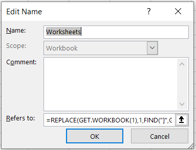
As for the 'Refers to' part, we will input a formula =REPLACE(GET.WORKBOOK(1),1, FIND("]," GET.WORKBOOK(1)), "") here, as illustrated below:

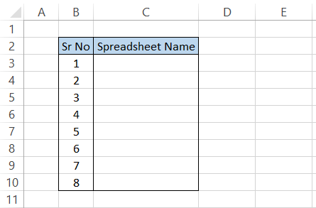
Click on Ok, and head to the spreadsheet, where you must return all the spreadsheet names in the workbook. Next, create a table with serial numbers as below:

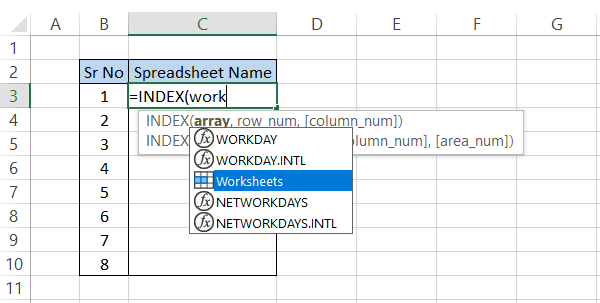
In cell C3, we will type the formula as =INDEX(worksheets, B3). The 'worksheets' is the named range we had created earlier, while the serial numbers work as an index assigned to each spreadsheet.

Once you drag the formula down to cell C10, we get the result.

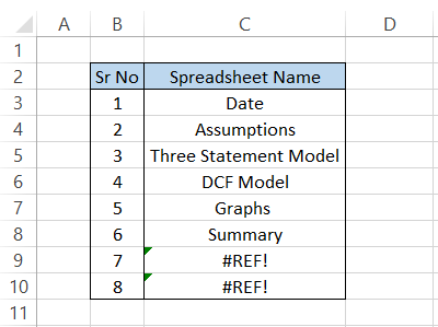
Since we do not have any sheets beyond the 'Summary' spreadsheet, Excel returns the #REF! Error. If new sheets are added to the workbook, drag down the formula again from cell C3 instead of making manual calculations using the F9 key.

Finally, we will explain why this method is useful. This enables us to create a table similar to the contents table and, further on, add hyperlinks to jump directly onto the respective page.

For example, in cell D3, we will use the formula =HYPERLINK("#'" &C3&" '!A1", "Go To Sheet") and drag it down till cell D10, which gives the result as:

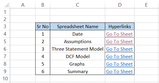
Now, clicking on any hyperlinks will directly jump to the selected sheet. Imagine this method's usefulness if you had hundreds of spreadsheets in the workbook.

If you need a backlink to the first sheet on each of the spreadsheets, follow the steps below:

• Create a hyperlink on the main page using the formula =HYPERLINK("#Date!A1","Main Page").
• This means we are hyperlinking the A1 cell of the Date spreadsheet, which is the first in our sequence.

• Copy the contents in cell A1. Next, select all the spreadsheets and use the ‘fill across the spreadsheet’ option from the Home tab. This way, you will find the backlink to the Main page in each spreadsheet and can easily navigate to the first page if required.

• Clicking on the hyperlink will directly take you to the first sheet in the workbook.

Sheet Name using VBA:

If you have been working on many projects recently where you need to type in the sheet names and add a hyperlink beside them, a VBA code will help you automate the workflow, potentially saving you hours.

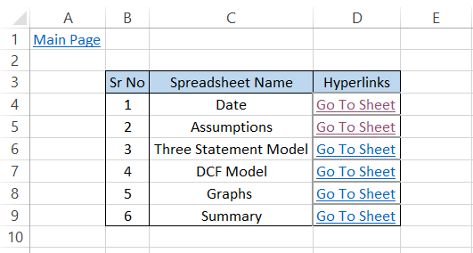
Suppose you are looking to write code for building a spreadsheet summary table as illustrated below:

The VBA code will include snippets that will evaluate the total number of spreadsheets along the names and return the result in the summary table. The code will look like this:

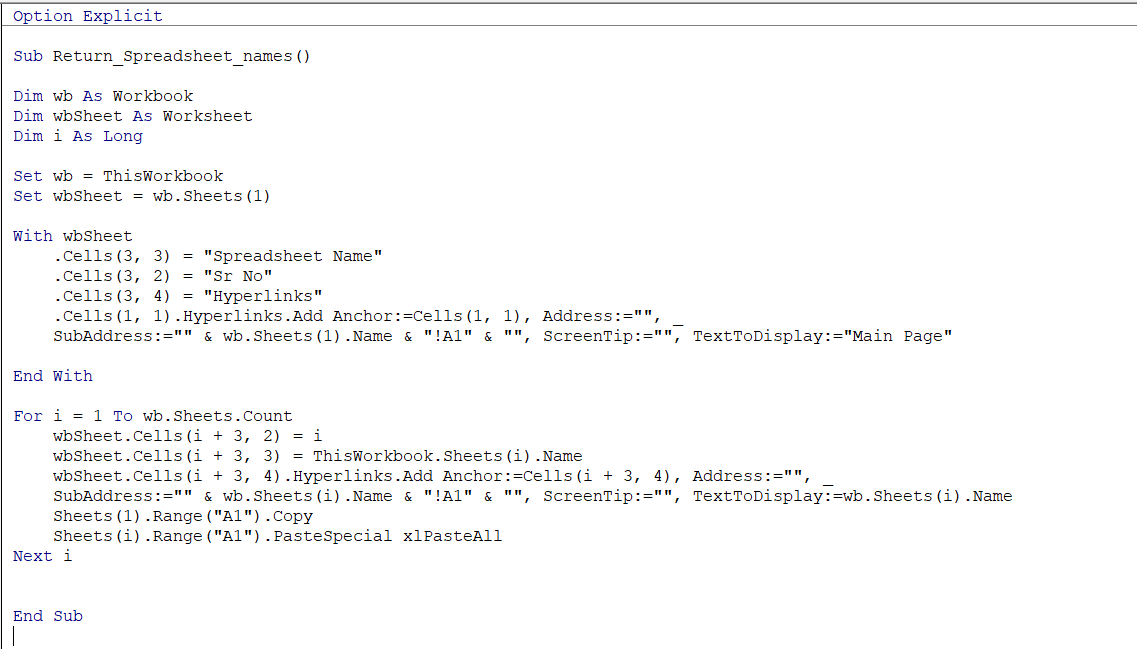
The code runs a loop that identifies the spreadsheet names, adds them to column C, and adds a hyperlink for the separate spreadsheets in column D.

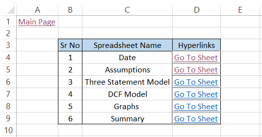
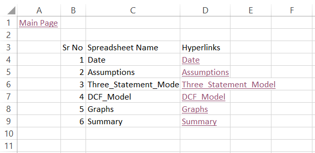
Thus, when you run the code by pressing the F5 key in the VBA Project window, you will get a summary table in Sheet1, as illustrated below:

This is quite similar to what we had built earlier. You could add a few lines of code to format the table, add a color fill for the headers, and input the border around the table.

With VBA, customizations are unlimited; however, you need to consider what you are building. Writing VBA code can sometimes be exhausting, but once you master this skill, no one will stop you.

Free Resources

To continue learning and advancing your career, check out these additional helpful WSO resources:

• Index Match Formula
• MOD Function
• REPLACE Function
• Scatter Plot
• Secondary Axis